Reading a Market Curve
How to read a market curve in the OpenTRMS Workbench — the tenor axis out to ten years, switching curve type, comparing two curves, and exporting values.
Transcript1m 36s
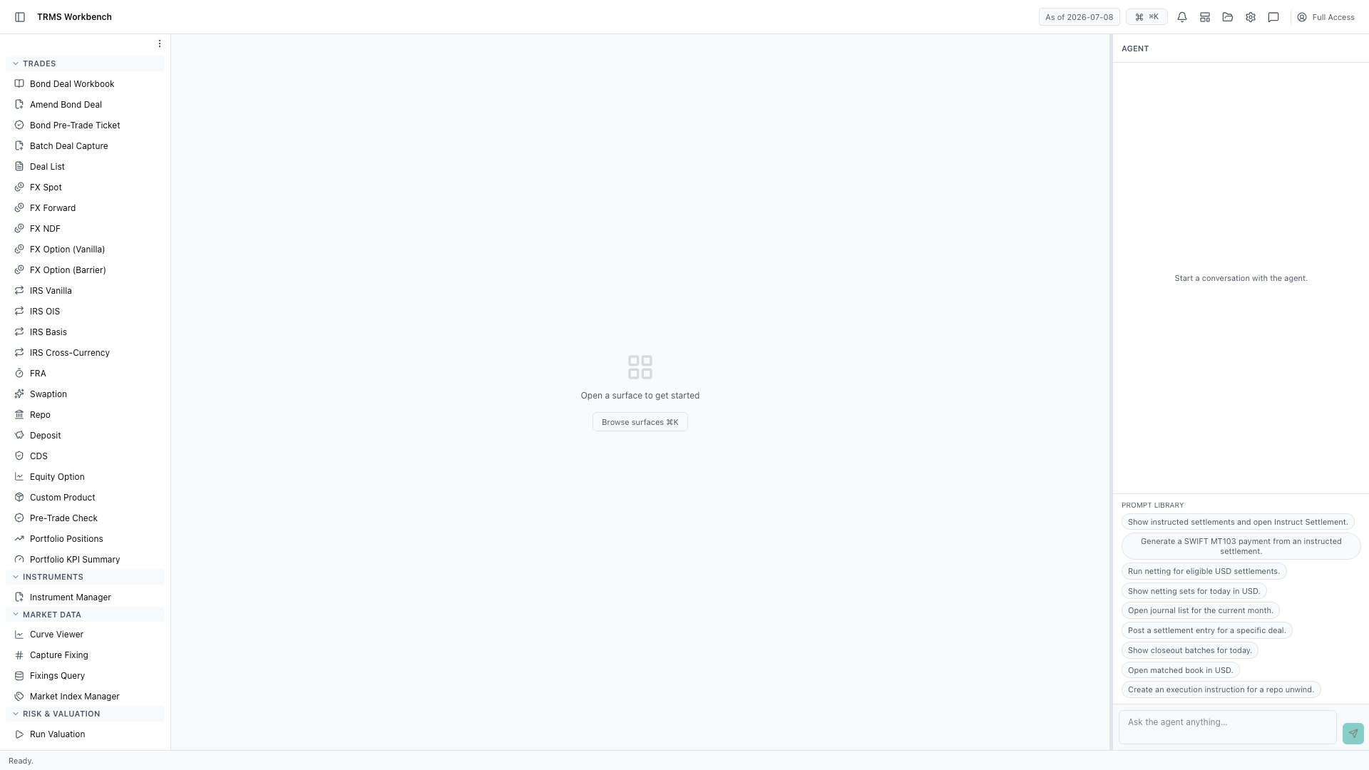
In this walkthrough we'll read a market curve, compare it with another, and export the values, in the OpenTRMS Workbench.
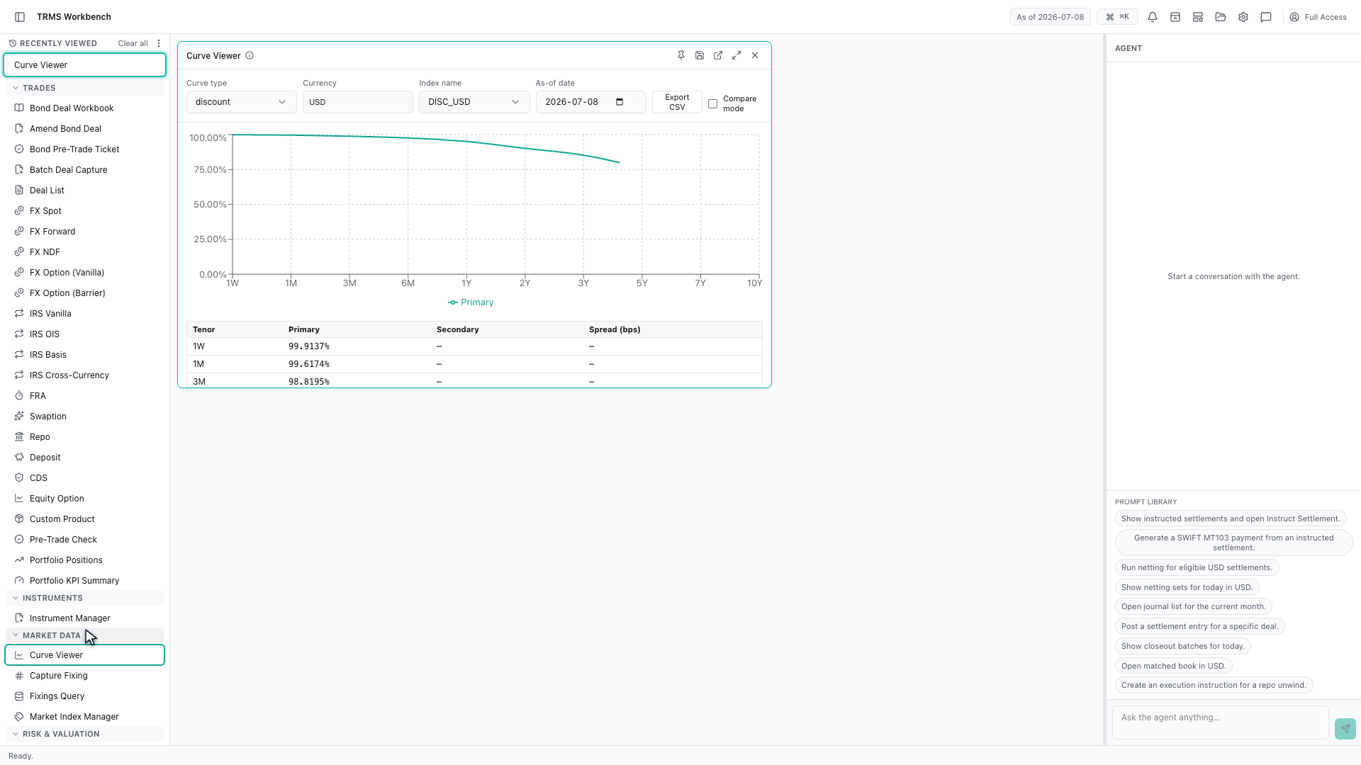
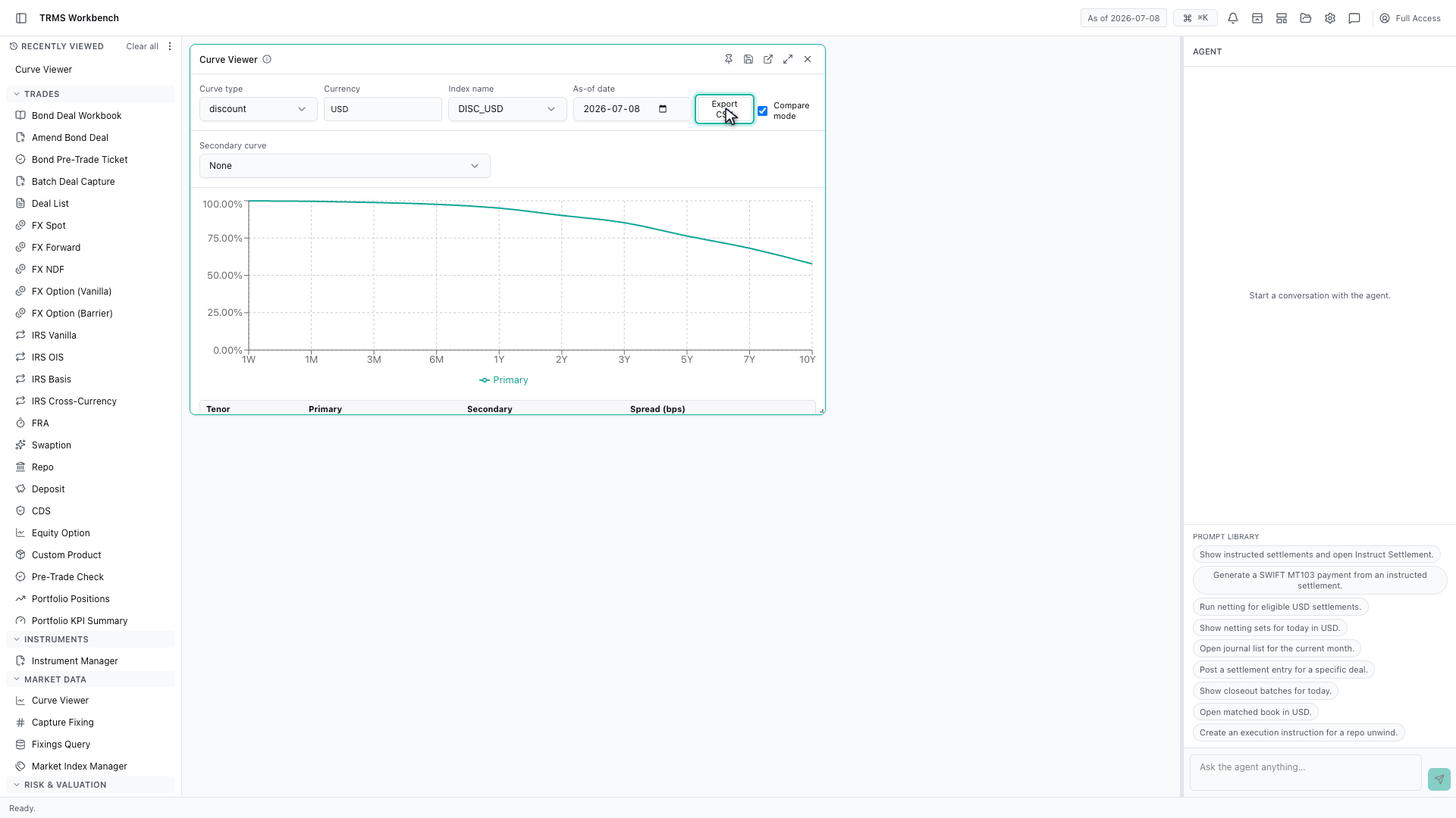
The Curve Viewer plots market curves by tenor. It opens on the US dollar discount curve, which is the one most other numbers are built from.
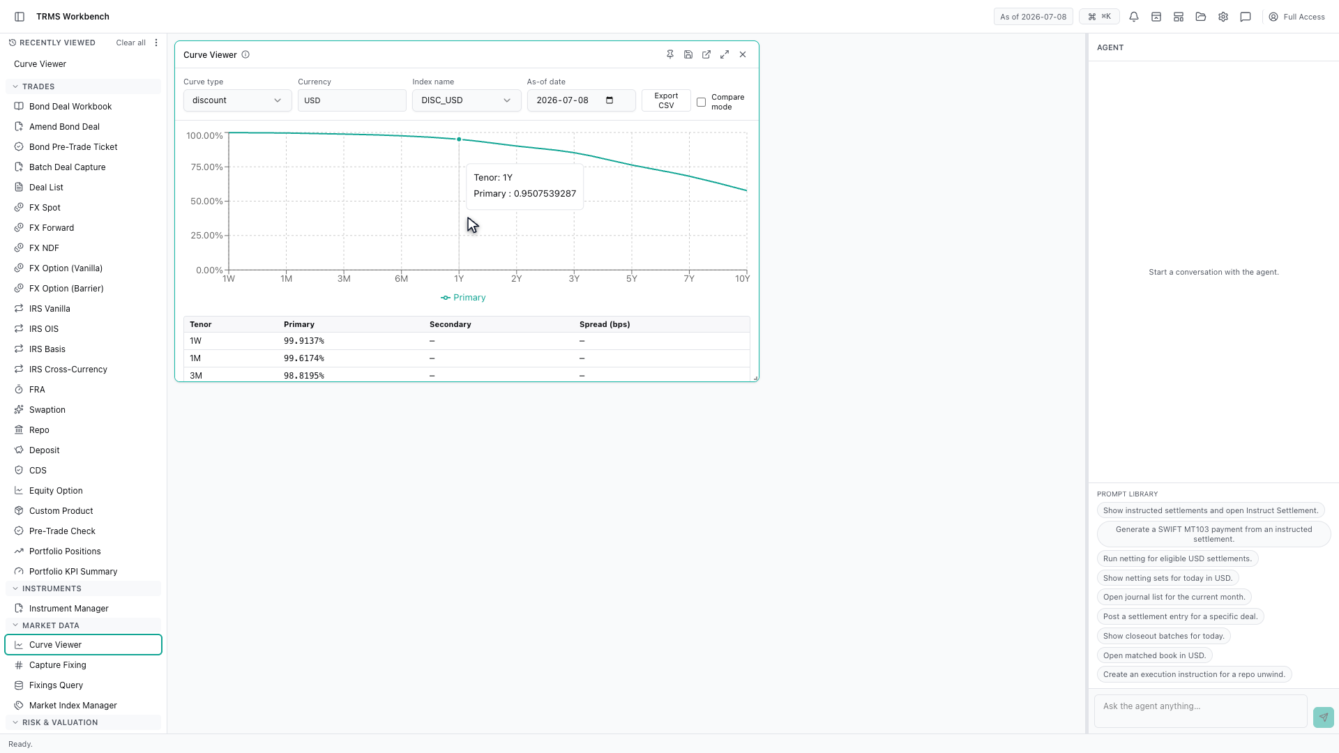
The horizontal axis is tenor, not calendar time. It runs from one week at the short end out to ten years at the long end, so the whole shape of the curve is on screen at once.
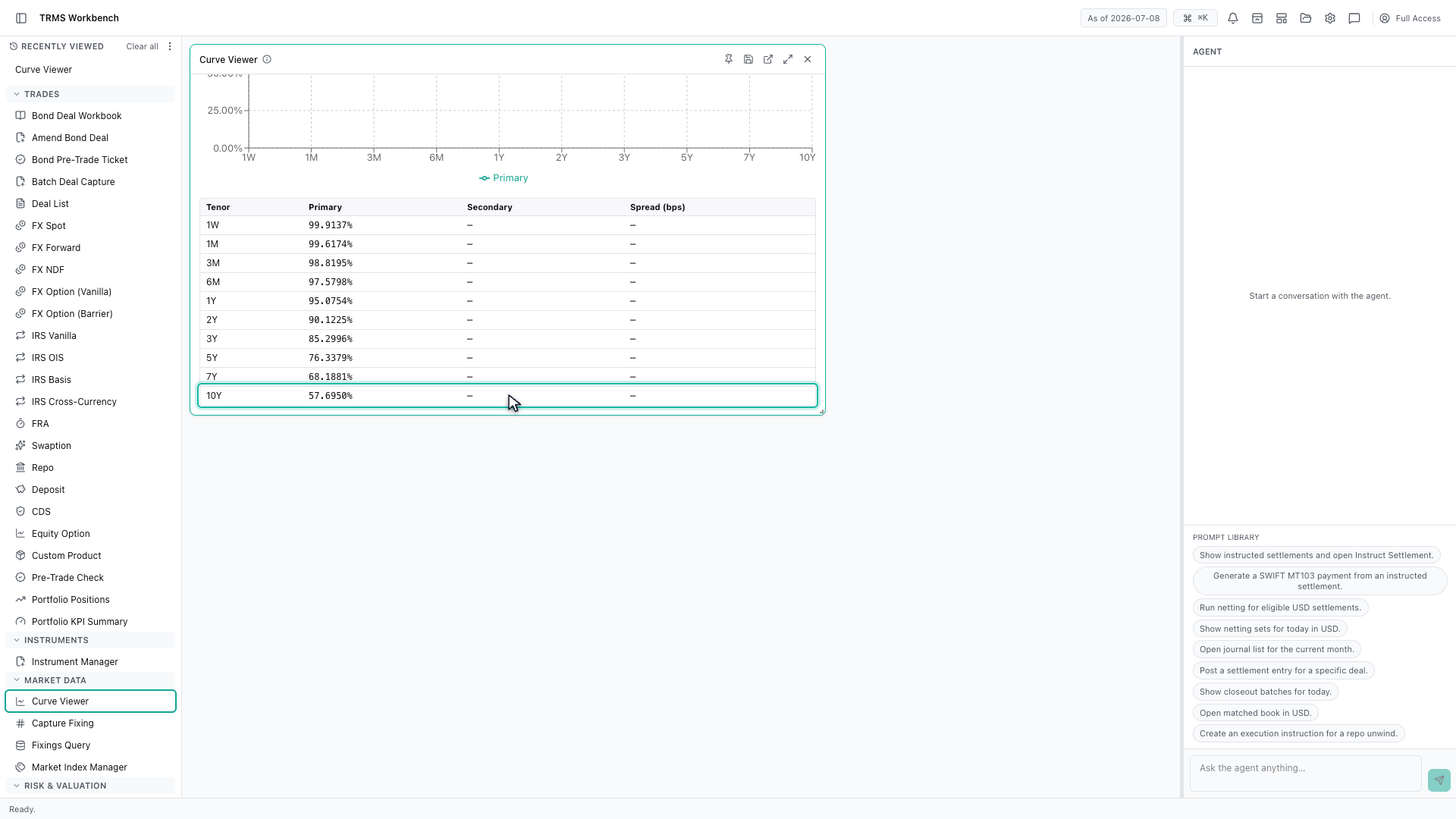
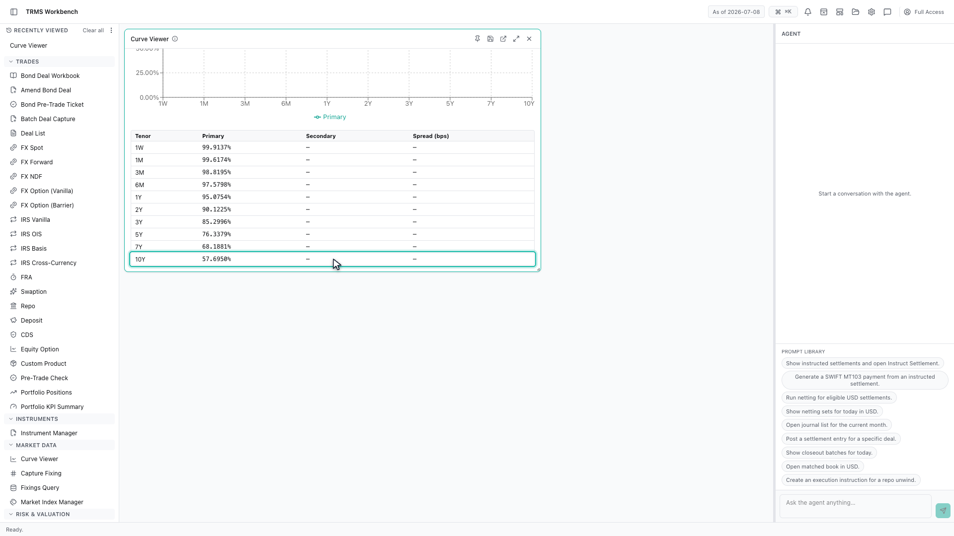
Underneath, the same curve is listed as numbers. This is where you read a specific point — the ten-year discount factor, for instance, rather than estimating it off the chart.
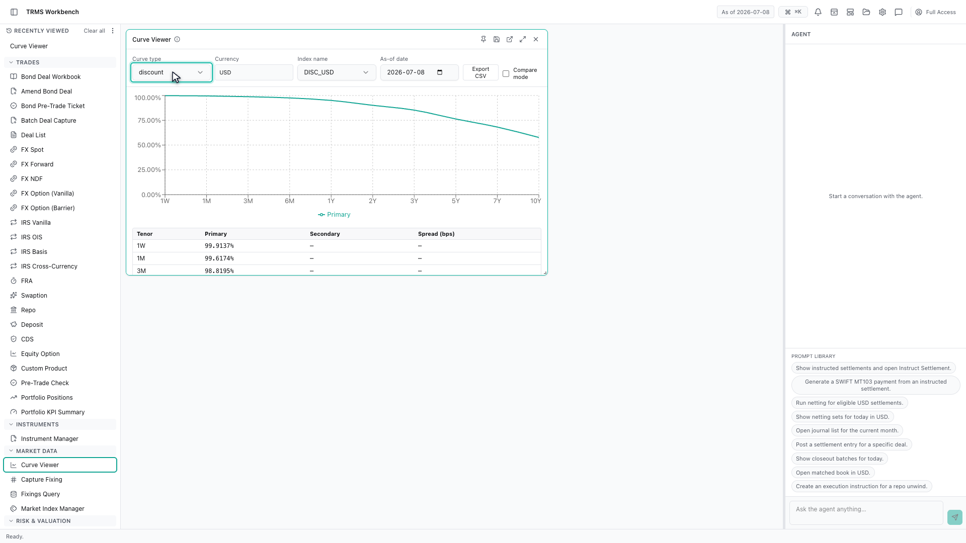
Curve type selects what is being plotted. Alongside discount there are yield, forward, projection, overnight index and credit curves, each built from the same market data.
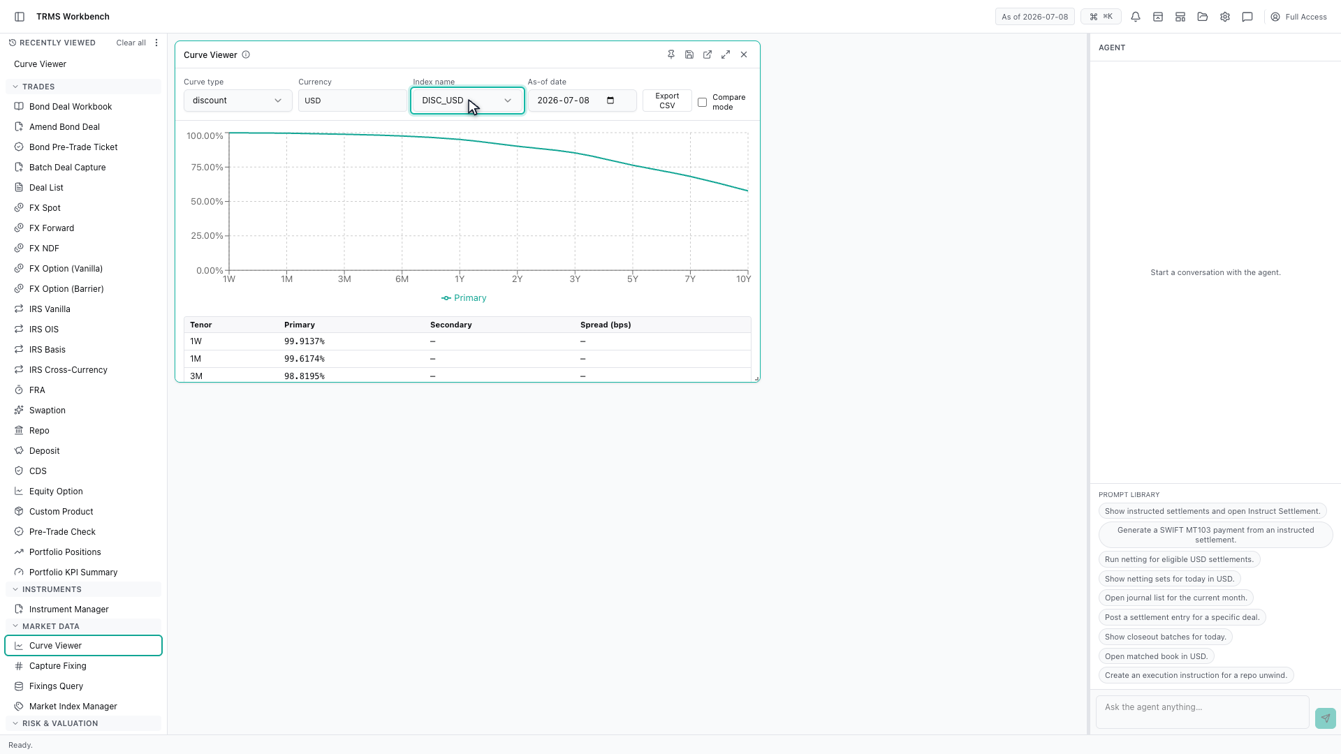
The index beside it picks which published curve to draw, and the as-of date decides which day's market data it is built from.
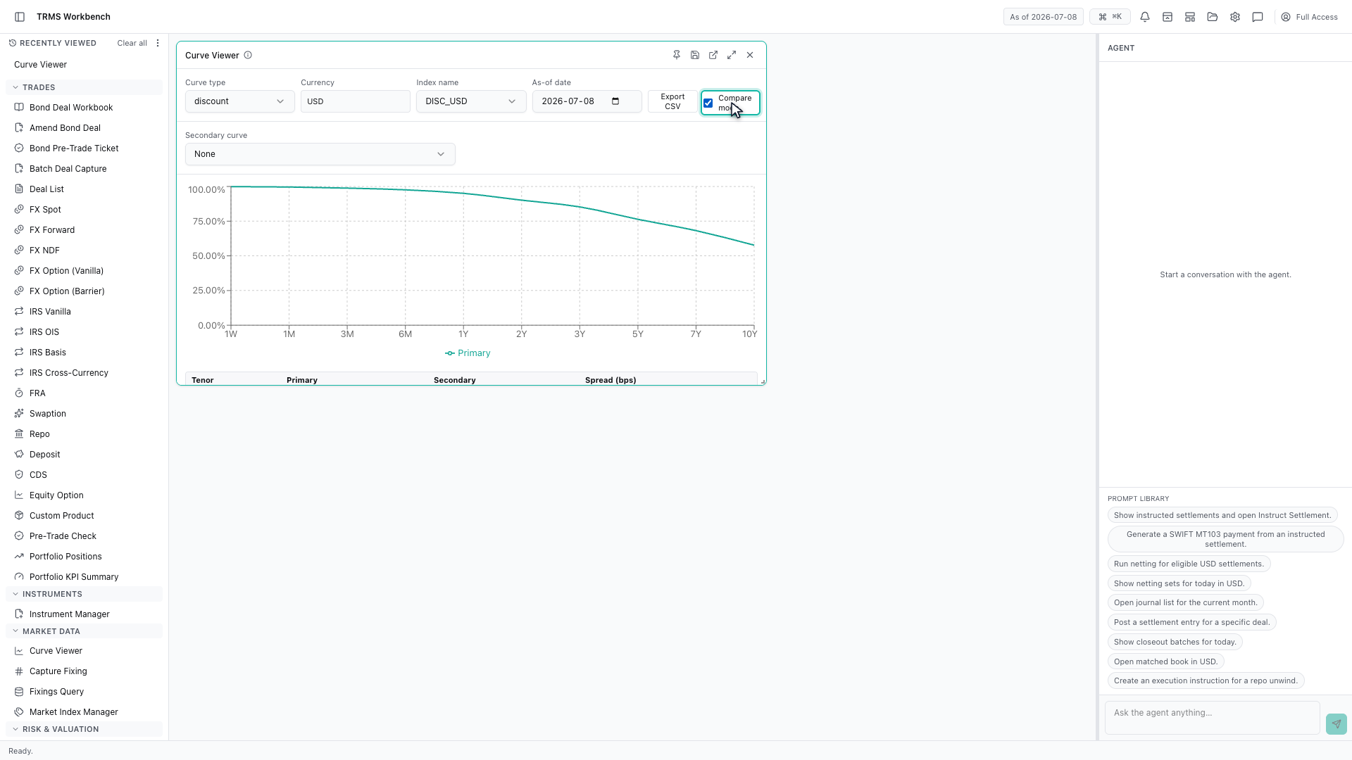
Compare mode puts a second curve alongside the first.
The table gains a secondary column and a spread in basis points, which is how you see the difference between two curves tenor by tenor rather than by eye.
And Export CSV takes the whole table out, so the same numbers can be checked or reused outside the Workbench.
That completes Reading a Market Curve. Every surface shown here can also be opened from the agent panel on the right, by asking for it in plain English.
1. Open the Workbench
In this walkthrough we'll read a market curve, compare it with another, and export the values, in the OpenTRMS Workbench.
2. Open the Curve Viewer
The Curve Viewer plots market curves by tenor. It opens on the US dollar discount curve, which is the one most other numbers are built from.
3. The tenor axis, one week to ten years
The horizontal axis is tenor, not calendar time. It runs from one week at the short end out to ten years at the long end, so the whole shape of the curve is on screen at once.
4. Read the ten-year point
Underneath, the same curve is listed as numbers. This is where you read a specific point — the ten-year discount factor, for instance, rather than estimating it off the chart.
5. Choose the curve type
Curve type selects what is being plotted. Alongside discount there are yield, forward, projection, overnight index and credit curves, each built from the same market data.
6. Choose the index and as-of date
The index beside it picks which published curve to draw, and the as-of date decides which day's market data it is built from.
7. Turn on compare mode
Compare mode puts a second curve alongside the first.
8. Read the spread between two curves
The table gains a secondary column and a spread in basis points, which is how you see the difference between two curves tenor by tenor rather than by eye.
9. Export the values
And Export CSV takes the whole table out, so the same numbers can be checked or reused outside the Workbench.
10. Next steps
That completes Reading a Market Curve. Every surface shown here can also be opened from the agent panel on the right, by asking for it in plain English.